
Data Validation (on the Data ribbon tab) is a handy feature to help maintain the integrity of your data. When providing a worksheet to your users, you want to be sure that they are providing appropriate data. For example, for a given cell, you may want to enforce conditions such as:
- Must be an integer between 1 and 100
- Must be a valid date after 1-Jan-2021
- Must be a value from a pre-defined list
These are very easy to set up simply using the Data Validation dialogue. Let’s try something a little more complex. What if we wanted to have more than one value-list data validation rule in which a selection from the first list of values determines which values are selectable in a secondary data validation list.
Consider the following scenario. We want to ask the user in one cell to choose one of the following region:
- West
- Central
- East
Based on their selection, we want to only list cities that pertain to the chosen region. For example:
| West | Central | East |
| Vancouver | Toronto | Fredericton |
| Calgary | Ottawa | Halifax |
| Edmonton | Montreal | St John’s |
| Winnipeg |
Assume that somewhere in your workbook that you have entered these lists
Steps:
- Create a named range containing the regions. For example, let’s name it Regions
- Create a named range for each of the cities listed above. The named ranges MUST match the items in the Regions list. Once completed, you should have three named ranges called West, Central and East.
- Set up Data Validation for the Regions on your worksheet. Assume that in our case, we created this Data Validat
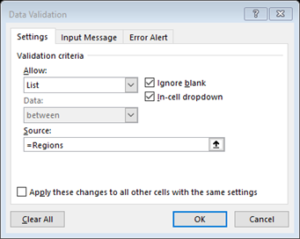 ion for cell A3
- In another cell set up Data Validation as shown. Note the use of the INDIRECT function in the Source
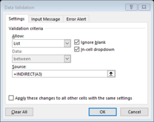 field
field
- Done
 !
!
What if your data validation list contains spaces? Using a similar scenario of regions and city data validation, assume the regions appear as:
- Western Region
- Central Region
- Eastern Region
Excel does not allow names ranges that contain spaces. A simple solution is to create named ranges from the validation lists omitting the spaces. Based on the above list of regions, create named city ranges as follows:
- WesternRegion
- CentralRegion
- EasternRegion
Then on the data validation for the cities, the formula becomes
=Indirect(Substitute($A$3, “ “,””))
The Substitute function will replace spaces in the selected region with an empty string. For example, a selected region of Western Region changes to WesternRegion which matches the named range. Then, as in the first example above, that named range is passed to the Indirect function.
In the sample file (click here), I include a second sheet that shows 2 additional means of creating cascading data validations. These examples are somewhat more involved but there are comments in the sheet to assist you.