MS Project is the premier project management tool, but it may be overkill to list a series of tasks to be performed with relative time frames and durations. Let’s assume we want to create a simplified Gantt chart, without using MS Project.
Key Features:
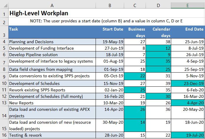
- Tasks Sheet – list of tasks within a project. The user can specify a task start date and one of the following. The remaining two attributes will automatically be calculated:
- Business days duration
- Calendar days duration
- Task end date
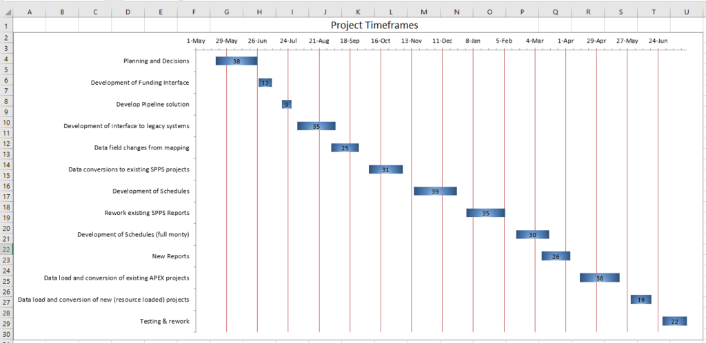
- Gantt Chart Sheet – Excel chart in a Gantt format
- Exception Dates Sheet – List of office closure dates
Building the Data Table
- Create and save a macro-enabled workbook with 3 sheets named as follows:
- Tasks
- Gantt Chart
- Exception Dates
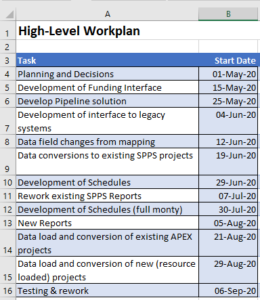
- On the Tasks sheet, add the following column headings (similar to that shown here):
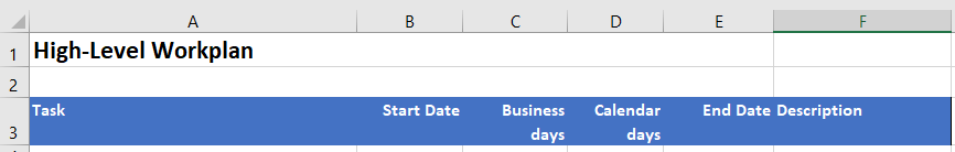
- Convert these headings to a table (In our scenario, select A3:F3 and Home -> Format as Table). Name the table TasksTable
- Select the range B4:E4 and create a named range called DatesAndDays
- Provide a list of tasks under the Tasks column and dates under the Start Dates column.
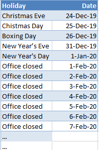
- On the Exception Dates sheet, create a table named ExceptionDates with one of the columns named Date. Enter a list of dates that are non-business dates (office closures, holidays, etc.)
- Add the following code to the Tasks worksheet
Note: the Description column is optional.
Note 1: Ensure you specify My table has headers 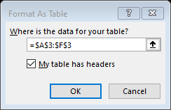
Note 2: I recommend you turn off filters on the table (Click Filter on the Data tab)
Note: The start dates can easily be changed later.
Building the Chart
Note: Values for business days and end date columns are not required initially. Ensure that each task has a start date and calendar days value. (These can be changed later).
- Select the first 2 columns (Task and Start Date), including the column labels (A3:B16 in this example)

- From the Insert tab, choose 2-D Stacked Bar chart type
- Right-click on the chart and choose Select Data

- Add another series

- Click on the series Add button
- Series name=Calendar Days (or click the cell with the Calendar Days column header)
- Series values = select the range of calendars days values
- Click OK
- Delete the legend if it was created. The chart should at this point look something like:

- Right-click on one of the bars of the start date series on the graph (blue bars above), and choose Format Data Series.

- Set the fill to No Fill
- Set border color to No Line
- Reverse the order of the tasks
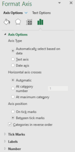
- Right-Click on the tasks list and choose Format Axis
- Click the Categories in Reverse Order (under Axis Position)
- Format the X-Axis
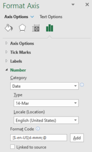
- Click on the X-axis values (dates) and choose Format Axis
- Select a desired date format (e.g. dd-mmm)
- At this point, cut the chart and paste it on the Gantt Chart sheet and then resize appropriately
- Create two named ranges on the Tasks sheet (for example in calls F1 and F2)
- MinRange – formula: =MIN(B:B)
- MaxRange – formula: =MAX(E:E)
- Remove the leading single quote from the following line in the code entered previously:
- ‘Call CalcScale … change to CalcScale
The Gantt chart is now ready to use and all that remains is the fine tuning of colours, bar widths, etc. according to taste. The user specifies tasks and Start dates. When the user enters either a number of Business days, number of Calendar days or an EndDate, those cells are shaded to indicate which cell was changed, formulas are built for the other cells between columns C to E, and the chart on the Gantt Chart sheet automatically re-builds as each task is updated and/or new tasks are added.
Click here to download the final solution.