
![]() To hide the ribbon when opening a workbook, add this VBA code to the Workbook object:
To hide the ribbon when opening a workbook, add this VBA code to the Workbook object:
Application.ExecuteExcel4Macro “SHOW.TOOLBAR(“”Ribbon””,False)”
![]() To hide the formula bar when opening a workbook, add this VBA code to the Workbook_Open event:
To hide the formula bar when opening a workbook, add this VBA code to the Workbook_Open event:
Application.DisplayFormulaBar = False
Note that you should also include the statement Application.DisplayFormulaBar=True in the Workbook_BeforeClose event
![]() To select all the cells on a worksheet, click the top left corner of the sheet (left of Column A and above row 1), or press Ctrl + A
To select all the cells on a worksheet, click the top left corner of the sheet (left of Column A and above row 1), or press Ctrl + A
![]() If you want to insert multiple rows, first highlight the desired number of rows after the row where the insertion is to take place. For example, if you wanted to insert 3 rows before row 3, first select rows 3, 4 and 5. Right-click on the row header column and choose Insert. Three rows will be inserted…. The prior row 3 is now row 6.
If you want to insert multiple rows, first highlight the desired number of rows after the row where the insertion is to take place. For example, if you wanted to insert 3 rows before row 3, first select rows 3, 4 and 5. Right-click on the row header column and choose Insert. Three rows will be inserted…. The prior row 3 is now row 6.
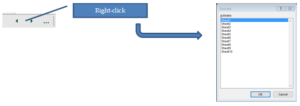
![]() Right-click on the bottom left navigation box left of the first sheet to show a list of all the sheets in the workbook. Double-click on an item in the list to launch that worksheet.
Right-click on the bottom left navigation box left of the first sheet to show a list of all the sheets in the workbook. Double-click on an item in the list to launch that worksheet.
![]() To scroll the list of worksheet tabs to the Last or First sheet, hold down the Shift or Tab keys and click the right or left navigation buttons in the bottom left navigation box (as mentioned in the prior hint). Only the list of sheet tabs will scroll… you remain on the active sheet.
To scroll the list of worksheet tabs to the Last or First sheet, hold down the Shift or Tab keys and click the right or left navigation buttons in the bottom left navigation box (as mentioned in the prior hint). Only the list of sheet tabs will scroll… you remain on the active sheet. ![]()
![]() Use Alt + Enter keys to enter multiple lines within a cell. Let’s say we need 3 lines of text within a cell as shown to the right. After the word “text”, hold down the Alt key, press Enter then type the next line of text.
Use Alt + Enter keys to enter multiple lines within a cell. Let’s say we need 3 lines of text within a cell as shown to the right. After the word “text”, hold down the Alt key, press Enter then type the next line of text.
![]() Format Painter (on the Home tab) provides a quick means to copy all the formatting (font, size, colours, alignment, etc.) from one area to another. Select a cell with formatting you would like to copy, click on Format Painter, then select a cell or range… the formatting is applied. If you double-click on Format Painter, the formatting can be copied to multiple selections of cells and ranges. The Painter remains active until you click Format Painter (to turn off)
Format Painter (on the Home tab) provides a quick means to copy all the formatting (font, size, colours, alignment, etc.) from one area to another. Select a cell with formatting you would like to copy, click on Format Painter, then select a cell or range… the formatting is applied. If you double-click on Format Painter, the formatting can be copied to multiple selections of cells and ranges. The Painter remains active until you click Format Painter (to turn off)
![]() The Clear function (on the Home tab) allows you to remove selective attributes of a cell or range. For example to remove all formatting (resetting everything back to the defaults), select the cell(s) and click the dropdown menu on the clear button and choose Clear Formats.
The Clear function (on the Home tab) allows you to remove selective attributes of a cell or range. For example to remove all formatting (resetting everything back to the defaults), select the cell(s) and click the dropdown menu on the clear button and choose Clear Formats.
![]() If you want to find all cells on a worksheet that contain formulas, conditional formatting, data validation, etc., click the Find & Select menu.
If you want to find all cells on a worksheet that contain formulas, conditional formatting, data validation, etc., click the Find & Select menu.
![]() You can add filter capability on select columns of data. Select the column heading(s) to enable filtering, click on Sort & Filter (on Home tab), choose Filter. Shortcut keys Ctrl+Shift+L turns on and off the filter function.
You can add filter capability on select columns of data. Select the column heading(s) to enable filtering, click on Sort & Filter (on Home tab), choose Filter. Shortcut keys Ctrl+Shift+L turns on and off the filter function.
![]() You can select and format multiple sheets together. Choose the first sheet, then
You can select and format multiple sheets together. Choose the first sheet, then
- If the remaining sheets are contiguous, hold down Shift then click the last sheet to be grouped
- If the remaining sheets are non-contiguous, hold down the Ctrl key and then select other sheets
Now any formatting changes on one sheet will be applied to all the sheets in the group
![]() You can drag and drop sheet tabs to re-order worksheets
You can drag and drop sheet tabs to re-order worksheets